How Can Creat Pie Chart.

The pie chart is one of the best excel features. It is used to visualize the contribution of each value to a complete pie diagram. It always uses one data series.
Follow the below steps to create a pie chart:
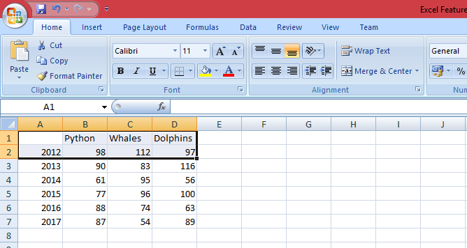
  • Select the range A1: D2.
MS Excel Features
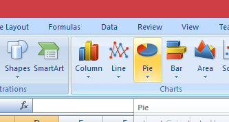
  • Now On the Insert tab, in the Charts group, click the Pie symbol and then click Pie.
TOP 10 Excel
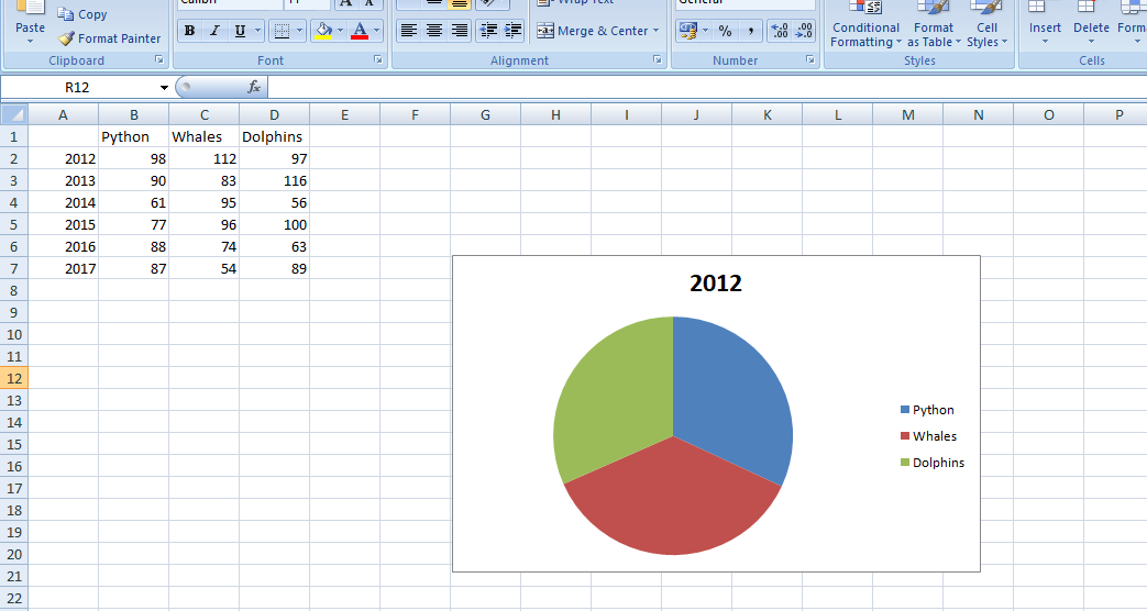
  • After clicking, the following image will show the result.
Microsoft Excel Features
The above figure shows us the pie chart for the year 2012. It is showing us the Python slice, Whales slice, and Dolphins slice. In short, the contribution of each slice.

Comments

Interactive Blogposts

рдиेрд▓्рд╕рди рдоंрдбेрд▓ा

рдордИ 2008 рдоें рдоंрдбेрд▓ा рджрдХ्рд╖िрдг рдЕрдл्рд░ीрдХा рдХे рд░ाрд╖्рдЯ्рд░рдкрддि рдкрдж рдмрд╣ाрд▓ 10 рдордИ 1994 – 14 рдЬूрди 1999 рд╕рд╣ाрдпрдХ рдеाрдмो рдо्рд╡ूрдпेрд▓рд╡ा рдо्рдмेрдХी рдПрдл рдбрдм्рд▓्рдпू рдбी рдХ्рд▓ेрд░्рдХ рдкूрд░्рд╡ा рдзिрдХाрд░ी рдПрдл рдбрдм्рд▓्рдпू рдбी рдХ्рд▓ेрд░्рдХ рдЙрдд्рддрд░ा рдзिрдХाрд░ी рдеाрдмो рдо्рд╡ूрдпेрд▓рд╡ा рдо्рдмेрдХी рдЬрди्рдо 18 рдЬुрд▓ाрдИ 1918   рдо्рд╡ेрдЬ़ो , рдХेрдк рдк्рд░ांрдд,  рджрдХ्рд╖िрдг рдЕрдл़्рд░ीрдХा рдоृрдд्рдпु 5 рджिрд╕рдо्рдмрд░ 2013 (рдЙрдо्рд░ 95) рд╣्рдпूрдЯрди,  рдЬोрд╣ाрди्рд╕рдмрд░्рдЧ , рджрдХ्рд╖िрдг рдЕрдл़्рд░ीрдХा рдЬрди्рдо рдХा рдиाрдо рд░ोрд▓ीрд╣्рд▓рд▓ा рдоंрдбेрд▓ा рд░ाрд╖्рдЯ्рд░ीрдпрддा рджрдХ्рд╖िрдг рдЕрдл़्рд░ीрдХी рд░ाрдЬрдиीрддिрдХ рджрд▓ рдЕрдл्рд░ीрдХрди рдиेрд╢рдирд▓ рдХांрдЧ्рд░ेрд╕ рдЬीрд╡рди рд╕ंрдЧी рдПрд╡рд▓िрди рдирдЯोрдХो рдоेрд╕ (рд╡ि 1944–1957; рддрд▓ाрдХ) рд╡िрдиी рдорджिрдХिрдЬ़ेрд▓ा (рд╡ि 1958–1996; рддрд▓ाрдХ़) рдЧ्рд░ाрд╢ा рдоैрдЪрд▓ (рд╡ि 1998–2013; рдоृрдд्рдпुрдкрд░्рдпंрдд) рдмрдЪ्рдЪे рдоेрдбिрдХा рдеेрдордмेрдХрд▓ рдоंрдбेрд▓ा рдоैрдХрдЬ़िрд╡ рдоंрдбेрд▓ा рдоैрдХрдЧाрдеो рд▓ेрд╡ाрдиिрдХा рдоंрдбेрд▓ा рдоैрдХрдЬ़िрд╡ рдоंрдбेрд▓ा рдЬ़ेрдиाрдиी рдоंрдбेрд▓ा рдЬ़िрдирдЬ़िрд╕्рд╡ा рдоंрдбेрд▓ा рдиिрд╡ाрд╕ рд╣्рдпूрдЯрди рдПрд╕्рдЯेрдЯ, рдЬोрд╣ाрдирд╕рдмрд░्рдЧ, рдЧौрдЯेंрдЧ, рджрдХ्рд╖िрдг рдЕрдл़्рд░ीрдХा рд╢ैрдХ्рд╖िрдХ рд╕рдо्рдмрдж्рдзрддा рдпूрдиिрд╡рд░्рд╕िрдЯी рдСрдл़ рдлोрд░्рдЯ рд╣ेрд░ рдпूрдиिрд╡рд░्рд╕िрдЯी рдСрдл़ рд▓ंрджрди рдПрдХ्рд╕рдЯрд░्рдирд▓ рд╕िрд╕्рдЯрдо рдпूрдиिрд╡рд░्рд╕िрдЯी рдСрдл़ рд╕ाрдЙрде рдЕрдл्рд░ीрдХा рдпूрдиिрд╡рд░्рд╕िрдЯी рдСрдл़ рдж рд╡िрдЯрд╡ाрдЯрд░рд╕्рд░ांрдб рдзрд░्рдо рдИрд╕ाрдИ ( рдоेрдеोрдбिрдЬ़्рдо ) рд╣рд╕्рддाрдХ्рд╖рд░ рдЬाрд▓рд╕्рдерд▓ www .nelsonmandela .org рдиेрд▓्рд╕рди рд░ोрд▓ीрд╣्рд▓рд▓ा рдоंрдбेрд▓ा  ( рдЦ़ोрд╕ा : N

Unsend Sent Messages

Unsend Sent Messages_ This is one of the most useful Gmail tricks. Go to   Settings  >  General tab  and check off “ Enable Undo Send .” You can also set the cancellation period as 5, 10, 20 or 30 seconds. Click on  Save Changes  at the bottom of the page. Next time when you send a message, you will see an  Undo  option in yellow below the search bar. You can click on it to unsend the message, and then you can edit it or discard it.

OFFSET combined with SUM or AVERAGE_#Yogendra

           OFFSET combined with SUM or AVERAGE Formula: =SUM(B4:OFFSET(B4,0,E2-1)) The OFFSET function on its own is not particularly advanced, but when we combine it with other functions like SUM or AVERAGE we can create a pretty sophisticated formula.  Suppose you want to create a dynamic function that can sum a variable number of cells.  With the regular SUM formula, you are limited to a static calculation, but by adding OFFSET you can have the cell reference move around. How it works:  To make this formula work, we substitute ending reference cell of the SUM function with the OFFSET function.  This makes the formula dynamic and the cell referenced as E2 is where you can tell Excel how many consecutive cells you want to add up. Now we’ve got some advanced Excel formulas! Below is a screenshot of this slightly more sophisticated formula in action. Add caption As you see, the SUM formula starts in cell B4, but it ends with a variable, which is the OFFSET f