1. Conditional Formatting

Making sense of our data-rich, noisy world is hard but vital. Used well, Conditional Formatting brings out the patterns of the universe, as captured by your spreadsheet. That's why Excel experts and Excel users alike vote this the #1 most important feature. This can be sophisticated. But even the simplest colour changes can be hugely beneficial. Suppose you have volumes sold by sales staff each month. Just three clicks can reveal the top 10% performing salespeople and tee up an important business conversation.
2. PivotTables
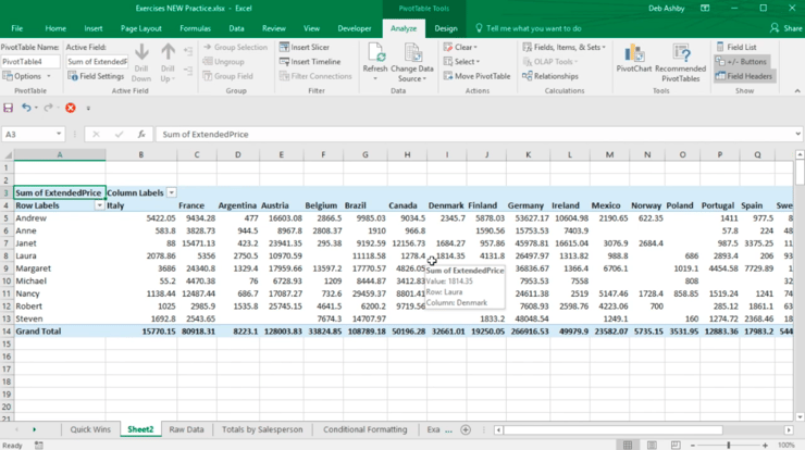
At 4 hours to get to proficiency, you may be put off learning PivotTables, but don't be. Use them to sort, count, total or average data stored in one large spreadsheet and display them in a n1ew table, cut however you want. That's the key thing here. If you want to look only at sales figures for certain countries, product lines or marketing channels, it's trivial. Warning: Make sure your data is clean first!
3. Paste Special
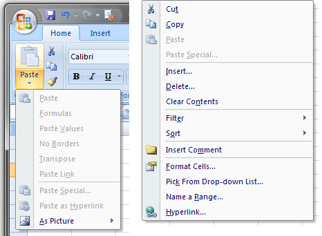 Grabbing (i.e. copying) some data from one cell and pasting it into another cell is one of the most common activities in Excel. But there's a lot you might copy (formatting, value, formula, comments, etc.) and sometimes you won't copy all of it. The most common example of this is where you want to lose the formatting. The place this data is going is your own spreadsheet with your own styling. It's annoying and ugly to plonk in formatting from elsewhere. So just copy the values and all you'll get is the text, number, whatever the value is. The shortcut after copying the cell (Ctrl C) is Alt E S V - easier to do than it sounds. The other big one is Transpose. This flips rows and columns around in seconds. Shortcut Alt E S E.
4. Add Multiple Rows
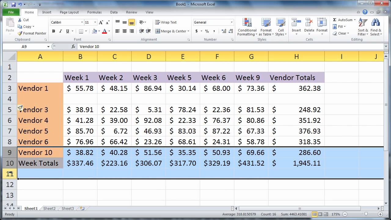
Probably one of the most frequently carried out activities in spreadsheeting. Ctrl Shift + is the shortcut, but actually it takes longer than just right-clicking on the row numbers on the left of the Excel display. So Right Click is our recommendation. And if you want to add more than one, select as many rows or columns as you'd like to add and then Right Click and add.
5. Absolute References
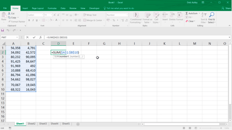
Indispensable! The dollar in front of the letter fixes the column, the dollar sign in front of number fixes the row, F4 toggles through the four possible combinations. Try it out with the following exercise. Type out three foods horizontally in cells B1, C1, D1 (Olives, Granola, Tomatoes) and three colours in cells A2, B2, C2 (Green, Blue, Yellow). Now type in cell B2 '=A2&" "&B1'. Congratulations: Green Olives! Now - and here's the exercise - add dollar signs so that when you copy the formula across you get green everything. Or just Granola, but of different colours. Experiment!
6. Print Optimisation
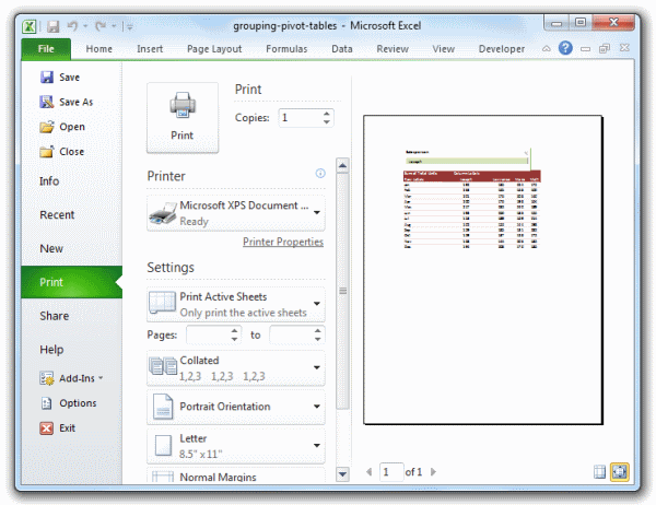
Everyone has problems printing from Excel. But imagine if what you printed were always just what you intended. It IS possible. But there are a few components to this: print preview, fit to one page, adjusting margins, print selection, printing headers, portrait vs landscape and spreadsheet design. Invest the time to get comfortable with it. You'll be carrying out this task many, many times in your working life.
7. Extend Formula Across/Down
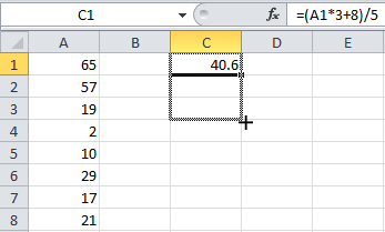 The beauty of Excel is its easy scalability. Get the formula right once and Excel will churn out the right calculation a million times. The + cross hair is handy. Double clicking it will take it all the way down if you have continuous data. Sometimes a copy and paste (either regular paste or paste formulas) will be faster for you.
8. Flash Fill
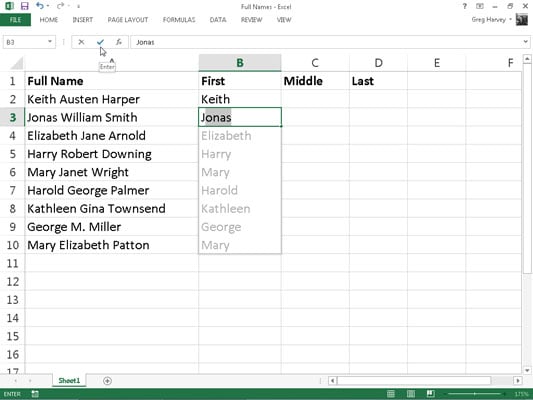 Excel developed a mind of its own in 2013. Say you have two columns of names and you need to construct email addresses from them all. Just do it for the first row and Excel will work out what you mean and do it for the rest. Pre-2013 this was possible but relied on a combination of functions (FIND, LEFT, &, etc). Now this is much faster and WILL impress people. If Flash Fill is turned on (File Options Advanced) it should just start working as you type. Or get it going manually by clicking Data > Flash Fill, or Ctrl E.
9. INDEX-MATCH

This is one of the most powerful combinations of Excel functions. You can use it to look up a value in a big table of data and return a corresponding value in that table. Let's say your company has 10,000 employees and there's a spreadsheet with all of them in it with lots of information about them like salary, start date, line manager etc. But you have a team of 20 and you're only really interested in them. INDEX-MATCH will look up the value of your team members (these need to be unique like email or employee number) in that table and return the desired information for your team. It is worth getting your head around this as it is more flexible and therefore more powerful than VLOOKUPs.
Comments
Post a Comment